Augmented Reality with Python and OpenCV (part 2)

The code of this project can be found here.

For those of you that have found this post before part 1 or that want to refresh what we have done up to this point, here you can catch up with the current state of the project so far. For the rest, we’ll keep going from where we left it. I’ve been really busy lately, so sorry if this second part is not as detailed as the first one.

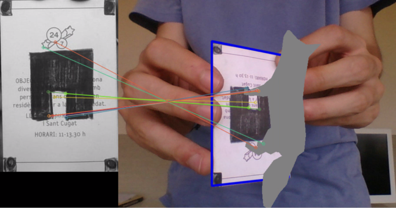
We left the project in a state where we were able to estimate the homography between our reference surface and a frame that contained that same surface in an arbitrary position. To do so we were using RANSAC. Well,  how do we keep building our augmented reality application from there?

Pose estimation from a plane

What we should achieve to project our 3D models in the frame is, as we have already said, to extend our homography matrix. We have to be able to project not only points contained in the reference surface plane (z-coordinate is 0), which is what we can do now, but any point in the reference space (with a z-coordinate different than 0).

If we go back to the first paragraphs of the section Homography Estimation, on part 1, we reached the conclusion that the 3×3 homography matrix was the product of the camera calibration matrix (A) by the external calibration matrix – which is an homogeneous transformation-. We dropped the third column (R3) of the homogeneous transformation because the z-coordinate of all the points we wanted to map was 0 (since all of them were contained in the reference surface plane). Figure 18 shows again the last steps of how we obtained the final expression of the homography matrix.

Figure 18: Derivation of the homography matrix. Source: F.Moreno

This meant that  we were left with the equation presented in Figure 19.

Figure 19: Components of the homography matrix. Source: F. Moreno

However, we now want to project points whose z-coordinate is different than 0, which is what will allow us to project 3D models. To do so we should find a way to compute, from what we know, the value of R3. Why? Because once z is different than 0 we can no longer drop R3 from the transformation (see Figure 18) since it is needed to map the z-value of the point we want to project. The problem of extending our transformation from 2D to 3D will be solved then when we find a way to obtain the value of R3 (see Figure 18, again). But, how can we get the value of R3?

We have already estimated the homography (H) , so its value is known. Furthermore, either by looking up the camera parameters or with a bit of common sense, we can easily know or make an educated guess of the values of the camera calibration matrix (A). Remember that the camera calibration matrix was:

Figure 20: Camera calibration matrix. Source: F. Moreno

Here you can find a nice article (part 3 of a recommended series) that talks in detail about the camera calibration matrix and each of its values, and you can even play with them. Since all I am building is a prototype application I just made an educated guess of the values of this matrix. When it comes to the projection of the optical center, I just set u0 and v0 to be half the resolution of the frames I am capturing with OpenCV (u0=320 and v0=240). As for the focal length, this article provides some useful information on how to estimate the focal length of a webcam or a cellphone camera. I set fu and fv to the same value, and found that a focal length of 800 worked quite well for me. You may have to adjust these parameters to your actual set up or even go on calibrating your camera.

Now that we have estimates of both the homography matrix H and our camera calibration matrix A, we can easily recover R1, R2 and t by multiplying the inverse of A by H:

Figure 21: Recovering the external calibration matrix values from the estimated homography and the camera calibration matrix. Source: F.Moreno

Were the values of G1, G2 and G3 can be regarded as:

Figure 22: Extracting the values of the external calibration matrix. Source: F.Moreno

Now, since the external calibration matrix [R1 R2 R3 t] is an homogeneous transformation that maps points amongst two different reference frames we can be sure that [R1 R2 R3] have to be orthonormal. Hence, theoretically we can compute R3 as:

Figure 23: Computation of R3. Source: F. Moreno

Unluckily for us, getting the value of R3 is not as simple as that. Since we obtained G1, G2 and G3 from estimations of A and H there is no guarantee that [R1=G1 R2=G2 R3=G1xG2] will be orthonormal. The problem is then to get a pair of vectors that are close to G1 and G2 (since G1 and G2 are estimates of the real values of R1 and R2) and that are orthonormal. Once this pair of vectors has been found (R1′ and R2′) then it will be true that R3 = R1’xR2′, so finding the value of R3 will be trivial. There are many ways in which we can find such a basis, an I will explain on of them. Its main benefit, from my point of view, is that it does not directly include any angle-related computation and that, once you get the hang of it, it is quite straightforward.

Finally and before diving into the explanation, the fact that the vectors we are looking for have to be close to G1 and G2 and not just any orthonormal basis in the same plane as G1 and G2 is important in understanding why some of the next steps are required. So make sure you understand it before moving on. I will try my best in explaining the process by which we will get this new basis but if don’t succeed in doing so do not hesitate to tell me and I will try to rephrase the explanation and make it clearer. It will be useful to have at hand Figure 24 since it provides visual information that can help in understanding the process. Note that what I am calling G1 and G2 are called R1 and R2 respectively in Figure 24. Let’s go for it!

We start with the reasonable assumption that, since G1 and G2 are estimates of the real R1 and R2 (which are orthonormal), the angle between G1 and G2 will be approximately 90 degrees (in the ideal case it will be exactly 90 degrees). Furthermore, the modulus of each of this vectors will be close to 1. From G1 and G2 we can easily compute an orthogonal basis -this meaning that the angle between the basis vectors will exactly be 90 degrees- that will be rotated approximately 45 degrees clockwise with respect to the basis formed by G1 and G2. This basis is the one formed by c=G1+G2 and  d = c x p = (G1+G2) x (G1 x G2) in Figure 24. If the vectors that form this new basis (c,d) are made unit vectors and rotated 45 degrees counterclockwise (note that once the vectors have been transformed into unit vectors – v / ||v|| – rotating the basis is as easy as d’ = c / ||c|| + d / ||d|| and  c’ = c / ||c|| – d / ||d||), guess what? We will have an orthogonal basis which is pretty close to our original basis (G1, G2). If we normalize this rotated basis we will finally get the pair of vectors we were looking for. You can see this whole process on Figure 24.

Figure 24: Normalization of [R1 R2 R3] to guarantee that they are orthonormal. Source: F.Moreno

Once this basis (R1′, R2′) has been obtained it is trivial to get the value of R3 as the cross product of R1′ and R2′.  This was tough, but we are all set now to finally obtain the matrix that will allow us to project 3D points into the image. This matrix will be the product of the camera calibration matrix A by [R1′ R2′ R3 t] (where t has been updated as shown in Figure 24). So, finally:

3D projection matrix = A · [R1′ R2′ R3 t]

Note that this 3D projection matrix will have to be computed for each new frame. With numpy we can, in a few lines of code, define a function that computes it for us:

def projection_matrix(camera_parameters, homography):
"""
 From the camera calibration matrix and the estimated homography
 compute the 3D projection matrix
 """
# Compute rotation along the x and y axis as well as the translation
homography = homography * (-1)
rot_and_transl = np.dot(np.linalg.inv(camera_parameters), homography)
col_1 = rot_and_transl[:, 0]
col_2 = rot_and_transl[:, 1]
col_3 = rot_and_transl[:, 2]
# normalise vectors
l = math.sqrt(np.linalg.norm(col_1, 2) * np.linalg.norm(col_2, 2))
rot_1 = col_1 / l
rot_2 = col_2 / l
translation = col_3 / l
# compute the orthonormal basis
c = rot_1 + rot_2
p = np.cross(rot_1, rot_2)
d = np.cross(c, p)
rot_1 = np.dot(c / np.linalg.norm(c, 2) + d / np.linalg.norm(d, 2), 1 / math.sqrt(2))
rot_2 = np.dot(c / np.linalg.norm(c, 2) - d / np.linalg.norm(d, 2), 1 / math.sqrt(2))
rot_3 = np.cross(rot_1, rot_2)
# finally, compute the 3D projection matrix from the model to the current frame
projection = np.stack((rot_1, rot_2, rot_3, translation)).T
return np.dot(camera_parameters, projection)

Note that the sign of the homography matrix is changed in the first line of the function. I will let you think why this is required.

As a summary, let me shortly recap our thought process to estimate the 3D matrix projection.

1. Derive the mathematical model of the projection (image formation). Conclude that, at this point, everything is an unknown.
2. Heuristically estimate the homography via keypoint matching and RANSAC. -> H is no longer unknown.
3. Estimate the camera calibration matrix. -> A is no longer unknown.
4. From the estimations of the homography and the camera calibration matrix along with the mathematical model derived in 1, compute the values of G1, G2 and t.
5. Find an orthonormal basis in the plane (R1′, R2′) that is similar to (G1,G2), compute R3 from it and update the value of t.

Figure 25: Thought process to recover the 3D projection matrix.

Model projection

Figure 26: Fox projection.

We are now reaching the final stages of the project. We already have all the required tools needed to project our 3D models. The only thing we have to do now is get some 3D figures and project them!

I am currently only using simple models in Wavefront .obj format. Why OBJ format? Because I found them easy to process and render directly with bare Python without having to make use of other libraries such as OpenGL. The problem with complex models is that the amount of processing they require is way more than what my computer can handle. Since I want my application to be real-time, this limits the complexity of the models I am able to render.

I downloaded several (low poly) 3D models format from clara.io such as this fox. Quoting Wikipedia, a .obj file is a geometry definition file format. If you download it and open the .obj file with your favorite text editor you will get an idea on how the model’s geometry is stored. And if you want to know more, Wikipedia has a nice in-detail explanation.

The code I used to load the models is based on this OBJFileLoader script that I found on Pygame’s website. I stripped out any references to OpenGL and left only the code that loads the geometry of the model. Once the model is loaded we just have to implement a function that reads this data and projects it on top of the video frame with the projection matrix we obtained in the previous section. To do so we take every point used to define the model and multiply it by the projection matrix. One this has been done, we only have to fill with color the faces of the model. The following function can be used to do so:

def render(img, obj, projection, model, color=False):
    vertices = obj.vertices
    scale_matrix = np.eye(3) * 3
    h, w = model.shape

    for face in obj.faces:
        face_vertices = face[0]
        points = np.array([vertices[vertex - 1] for vertex in face_vertices])
        points = np.dot(points, scale_matrix)
        # render model in the middle of the reference surface. To do so,
        # model points must be displaced
        points = np.array([[p[0] + w / 2, p[1] + h / 2, p[2]] for p in points])
        dst = cv2.perspectiveTransform(points.reshape(-1, 1, 3), projection)
        imgpts = np.int32(dst)
        if color is False:
            cv2.fillConvexPoly(img, imgpts, (137, 27, 211))
        else:
            color = hex_to_rgb(face[-1])
            color = color[::-1] # reverse
            cv2.fillConvexPoly(img, imgpts, color)

    return img

There are two things to be highlighted from the previous function:

1.  The scale factor: Since we don’t know the actual size of the model with respect to the rest of the frame, we may have to scale it (manually for now) so that it haves the desired size. The scale matrix allows us to resize the model.
2.  I like the model to be rendered on the middle of the reference surface frame. However, the reference frame of the models is located at the center of the model. This means that if we project directly the points of the OBJ model in the video frame our model will be rendered on one corner of the reference surface. To locate the model in the middle of the reference surface we have to, before projecting the points on the video frame, displace the x and y coordinates of all the model points by half the width and height of the reference surface.
3. There is an optional color parameter than can be set to True. This is because some models also have color information that can be used to color the different faces of the model. I didn’t test it enough and setting it to True might result in some problems. It is not 100% guaranteed this feature will work.

And that’s all!

Results

Here you can find some links to videos that showcase the current results. As always, there are many things that can be improved but overall we got it working quite well.

• Results 2
• Results 3
• Results 4
• Results 5
• Results 6
• Results 7

Final notes

Figure 27: Done. Let’s ship the code!

Especially for Linux users, make sure that your OpenCV installation has been compiled with FFMPEG support. Otherwise, capturing video will fail. Pre-built OpenCV packages such as the ones downloaded via pip are not compiled with FFMPEG support, which means that you will have to build it manually.

As usual, you can find the code of this project on GitHub. I would have liked to polish it a bit more and add a few more functionalities, but this will have to wait. I hope the current state of the code is enough to get you started.

The code might not work directly as-is (you should change the model, tweak some parameters, etc.), but with some tinkering you can surely make it work! I’ll try to help in any issues you find along the way!