Landscape generation using midpoint displacement

Today I will present how to implement in Python a simple yet effective algorithm for proceduraly generating 2D landscapes. It is called Midpoint Displacement (or Diamond-square algorithm, which seems less intuitive to me) and, with some tweaking it can also be used for creating rivers, lighting strikes or (fake) graphs. The final output may look like the following image.

Example terrain generated with the presented algorithm.

Algorithm overview

The main idea of the algorithm is as follows: Begin with a straight line segment, compute its midpoint and displace it by a bounded random value. This displacement can be done either by:

1. Displacing the midpoint in the direction perpendicular to the line segment.
2. Displacing only the y coordinate value of the midpoint.

Different methods for displacing the midpoint.

This first iteration will result in two straight line segments obtained from the displacement of the midpoint of the original segment.  The same process of computing and displacing the midpoint can be then applied to each of this new two segments and it will result in four straight line segments. Then we can repeat the process for each of this four segments to obtain eight and so on. The process can be repeated iteratively or recursively as many times as desired or until the segments cannot be reduced more (for graphical applications this limit would be two pixel’s width segments). The following image may help to clarify what I just said.

From top to bottom, successive iterations of the algorithm.

And that’s it! This is the core idea of the midpoint displacement algorithm. In pseudocode it looks like:

Initialize segment
While iterations < num_of_iterations and segments_length > min_length:
	For each segment:
		Compute midpoint
		Displace midpoint
		Update segments
        Reduce displacement bounds
        iterations+1

However, before implementing the algorithm we should dig deeper in some of the concepts that have arisen so far. These are mainly:

• How much should we displace the midpoint?
• How much should the displacement bounds be reduced after each iteration?

How much should we displace the midpoint?

Sadly, there is no general answer for this question because it greatly depends on two aspects:

1. The application the algorithm is being used for
2. The desired effect

Since in this post our scope is terrain generation I will limit the explanation to the effects that this parameter has in this area. However, the ideas that I will explain now can be extrapolated to any other application where the Midpoint Displacement algorithm may be used. As I see it, there are two key considerations that should be taken into account when deciding the initial displacement value.

First of all, we should consider which is the desired type of terrain. Hopefully it makes sense to say that the bigger the mountains we want to generate the bigger the initial displacement value should be and viceversa. With a bit of trial and error it is easy to get an idea of the average profiles generated by different values and how do they look. The point here is that bigger mountains need bigger initial displacement values.

Secondly,  the overall dimensions (width and height) of the generated terrain. The initial displacement should be regarded as a value which depends on the generated terrain dimensions.  What I want to say is that an initial displacement of 5 may be huge when dealing with a 5×5 image but will hardly be noticed in a 1500×1500 image.

The same initial displacement value may be to big for a certain image size but may suit well another image size.

How much should the bounds be reduced after each iteration?

Well, the answer again depends on which is the desired output. It should be intuitive that the smaller the displacement reduction the more jagged the obtained profile will be and viceversa. The two extremes are no displacement reduction at all and setting the displacement to 0 after the first iteration. This two cases can be observed in the figure below.

On the left: no displacement reduction. On the right: Displacement reduction to 0 after first iteration.

Somewhere in between is the displacement reduction that will yield the desired output. There are plenty of ways to reduce the displacement bounds each iteration (linearly, exponentially, logarithmically, etc.) and I encourage you to try different ones and see how the results vary.

What I did was define a standard displacement reduction of 1/2, which means that the displacement is reduced by half each new iteration,  and a displacement decay power i such that the displacement reduction is

displacement_reduction = 1/(2^i)

and

displacement_bounds(k+1) = displacement_bounds(k)*displacement_reduction

were k is the current iteration and k+1 the next iteration. We can then talk about the obtained terrain profiles in terms of this decay power i. Below you can see how the algorithm performs for different decay powers.

Obtained profiles for different values of  the displacement decay powers.

Bear in mind that the two factors we just saw, the bounds reduction and initial displacement are related one to the other and that they do not affect the output independently. Smaller initial displacements may look good with smaller decay powers and viceversa. Here we have talked about some guidelines that may help when deciding which values to use but there will be some trial and error until the right parametres for the desired output are found. Finally, the number of iterations is another factor that also affects the output in relation with the initial displacement and the bounds reduction.

Python implementation

Finally it is time to, with all the ideas explained above, code our 2D terrain generator. For this particular implementation I have decided to:

• Displace only the y coordinate of the midpoints (Second of the two displacement methods explained at the begining).
• Use symmetric bounds with respect to zero for the displacement (if b is the upper bound then –b will be the lower bound.)
• Choose the displacement value to be either the upper bound or the lower bound, but never allow values in between.
• Reduce the bounds after each iteration by multiplying the current bounds by 1/(2^i)

We will have three functions: one that will generate the terrain, one that will draw the generated terrain and one that will handle the above processes.

Before implementing the functions we should first import the modules that we will use:

import os                             # path resolving and image saving
import random                         # midpoint displacement
from PIL import Image, ImageDraw      # image creation and drawing
import bisect                         # working with the sorted list of points

Terrain generation

For the terrain generation we need a function that, given a straight line segment returns the profile of the terrain. I have decided to provide as inputs the initial segment and displacement, the rate of decay or roughness of the displacement and the number of iterations:

# Iterative midpoint vertical displacement
def midpoint_displacement(start, end, roughness, vertical_displacement=None,
                          num_of_iterations=16):
    """
    Given a straight line segment specified by a starting point and an endpoint
    in the form of [starting_point_x, starting_point_y] and [endpoint_x, endpoint_y],
    a roughness value > 0, an initial vertical displacement and a number of
    iterations > 0 applies the  midpoint algorithm to the specified segment and
    returns the obtained list of points in the form
    points = [[x_0, y_0],[x_1, y_1],...,[x_n, y_n]]
    """
    # Final number of points = (2^iterations)+1
    if vertical_displacement is None:
        # if no initial displacement is specified set displacement to:
        #  (y_start+y_end)/2
        vertical_displacement = (start[1]+end[1])/2
    # Data structure that stores the points is a list of lists where
    # each sublist represents a point and holds its x and y coordinates:
    # points=[[x_0, y_0],[x_1, y_1],...,[x_n, y_n]]
    #              |          |              |
    #           point 0    point 1        point n
    # The points list is always kept sorted from smallest to biggest x-value
    points = [start, end]
    iteration = 1
    while iteration <= num_of_iterations:
        # Since the list of points will be dynamically updated with the new computed
        # points after each midpoint displacement it is necessary to create a copy
        # of the state at the beginning of the iteration so we can iterate over
        # the original sequence.
        # Tuple type is used for security reasons since they are immutable in Python.
        points_tup = tuple(points)
        for i in range(len(points_tup)-1):
            # Calculate x and y midpoint coordinates:
            # [(x_i+x_(i+1))/2, (y_i+y_(i+1))/2]
            midpoint = list(map(lambda x: (points_tup[i][x]+points_tup[i+1][x])/2,
                                [0, 1]))
            # Displace midpoint y-coordinate
            midpoint[1] += random.choice([-vertical_displacement,
                                          vertical_displacement])
            # Insert the displaced midpoint in the current list of points         
            bisect.insort(points, midpoint)
            # bisect allows to insert an element in a list so that its order
            # is preserved.
            # By default the maintained order is from smallest to biggest list first
            # element which is what we want.
        # Reduce displacement range
        vertical_displacement *= 2 ** (-roughness)
        # update number of iterations
        iteration += 1
    return points

The initial line segment is specified by the coordinates of the points where it begins and ends. Both are a list in the form:

point = [x_coordinate, y_coordinate]

And the output is a list of lists containing all the points that should be connected to obtain the terrain profile in the form:

points = [[x_0, y_0], [x_1, y_1], ..., [x_n, y_n]]

Terrain drawing

For the graphical output we need a function that returns an image of the drawn terrain and that takes as inputs at least the profile generated by the midpoint displacement algorithm. I have also included as inputs the desired width and height of the image and the colors it should use for painting. What I did for drawing several layers of terrain was start with the layer in the background and draw each new layer on top of the previous one.

For drawing each layer I first infer the y value of every x value in the range (0, image width) based on the assumption that the known points, the ones obtained from the midpoint displacement, are connected with straight lines. Once knowing the y value of each x value in the range (0, image width) I traverse all the x values iteratively and for each x value draw a line from its y value to the bottom of the image.

def draw_layers(layers, width, height, color_dict=None):
    # Default color palette
    if color_dict is None:
        color_dict = {'0': (195, 157, 224), '1': (158, 98, 204),
                      '2': (130, 79, 138), '3': (68, 28, 99), '4': (49, 7, 82),
                      '5': (23, 3, 38), '6': (240, 203, 163)}
    else:
        # len(color_dict) should be at least: # of layers +1 (background color)
        if len(color_dict) < len(layers)+1:
            raise ValueError("Num of colors should be bigger than the num of layers")

    # Create image into which the terrain will be drawn
    landscape = Image.new('RGBA', (width, height), color_dict[str(len(color_dict)-1)])
    landscape_draw = ImageDraw.Draw(landscape)
    # Draw the sun
    landscape_draw.ellipse((50, 25, 100, 75), fill=(255, 255, 255, 255))
    # Sample the y values of all x in image
    final_layers = []
    for layer in layers:
        sampled_layer = []
        for i in range(len(layer)-1):
            sampled_layer += [layer[i]]
            # If x difference is greater than 1
            if layer[i+1][0]-layer[i][0] > 1:
                # Linearly sample the y values in the range x_[i+1]-x_[i]
                # This is done by obtaining the equation of the straight
                # line (in the form of y=m*x+n) that connects two consecutive
                # points
                m = float(layer[i+1][1]-layer[i][1])/(layer[i+1][0]-layer[i][0])
                n = layer[i][1]-m*layer[i][0]
                r = lambda x: m*x+n  # straight line
                for j in range(layer[i][0]+1, layer[i+1][0]):  # for all missing x
                    sampled_layer += [[j, r(j)]]  # Sample points
        final_layers += [sampled_layer]

    final_layers_enum = enumerate(final_layers)
    for final_layer in final_layers_enum:
        # traverse all x values in the layer
        for x in range(len(final_layer[1])-1):
            # for each x value draw a line from its y value to the bottom
            landscape_draw.line((final_layer[1][x][0], height-final_layer[1][x][1],
                                 final_layer[1][x][0], height),
                                 color_dict[str(final_layer[0])])

    return landscape

The PIL module (and mostly all the modules that allow working with images) sets the origin of coordinates on the top left corner of the image. Also, the x value increases when moving right and the y value when moving down. The y values that have to be passed to the function that draws the lines have to be expressed in this system of reference and that is why for drawing the desired line its y values have to be transformed from our reference system (origin lower left) to PIL’s reference system.

Differences between PIL’s reference system and the one we have been using so far.

With these two functions we are now able to actually compute and draw our 2D proceduraly generated terrain.

Our main function

The final step is to define our main function. This function will compute the profiles of the desired number of layers, draw them and save the obtained terrain as a .png image:

def main():
    width = 1000  # Terrain width
    height = 500  # Terrain height
    # Compute different layers of the landscape
    layer_1 = midpoint_displacement([250, 0], [width, 200], 1.4, 20, 12)
    layer_2 = midpoint_displacement([0, 180], [width, 80], 1.2, 30, 12)
    layer_3 = midpoint_displacement([0, 270], [width, 190], 1, 120, 9)
    layer_4 = midpoint_displacement([0, 350], [width, 320], 0.9, 250, 8)

    landscape = draw_layers([layer_4, layer_3, layer_2, layer_1], width, height)

    landscape.save(os.getcwd()+'\\testing.png')

To call the main() function when we run the program we finally add the lines:

if __name__ == "__main__":
    main()

And we’re done! Now it’s your turn to code your own terrain generator and play with its different parametres for modifying the results (you can also change the colors). If you have any doubts do not hesitate to contact me. You can find the whole code at github.

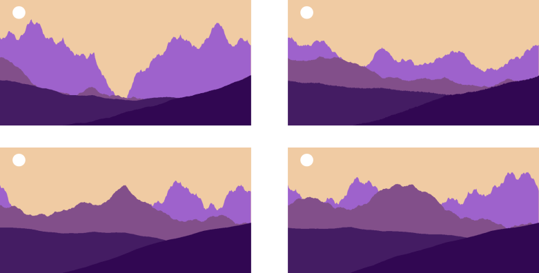
As a bonus, some more terrain images obtained with the previous code:

Midpoint Displacement 2D generated landscapes.